Constrained Sensing for Simulation of a Fuel Rod
This notebook explores the PySensors General QR GQR optimizer and the constraints class within utils for spatially-constrained sparse sensor placement (for reconstruction) of the temperature field within an electrically heated fuel rod prototype (OPTI-TWIST).
The General QR algorithm was devised specifically to solve such problems. The PySensors object implementing this method is named GQR and in this notebook we’ll demonstrate its use on a temperature field reconstruction problem.
In this notebook we particularly showcase the functionalities offered by the constraints class. For example, if the user provides the center and radius of a circular constrained region, the constraints in utils compute the constrained sensor indices. Direct constraint plotting capabilities have also been developed.
The constrained shapes currently implemented are: Circle, Cylinder, Line, Parabola, Ellipse, and Polygon
A user can define their own constrained shape using UserDefinedConstraints to take in either a function from the user or a .py file which contains a functional definition of the constrained region.
See the following reference for more information,
Karnik N, Abdo MG, Estrada-Perez CE, Yoo JS, Cogliati JJ, Skifton RS, Calderoni P, Brunton SL, Manohar K. Constrained optimization of sensor placement for nuclear digital twins. IEEE Sensors Journal. 2024 Feb 28. (link)
Karnik N, Wang C, Bhowmik PK, Cogliati JJ, Balderrama Prieto SA, Xing C, Klishin AA, Skifton R, Moussaoui M, Folsom CP, Palmer JJ, Sabharwall P, Manohar K, Abdo MG., Leveraging Optimal Sparse Sensor Placement to Aggregate a Network of Digital Twins for Nuclear Subsystems. Energies (19961073). 2024 Jul 1;17(13). (link)
[1]:
import matplotlib.pyplot as plt
import numpy as np
import warnings
warnings.filterwarnings('ignore')
import pysensors as ps
[2]:
from IPython.display import HTML
HTML("""
<style>
.output {
    display: flex;
    text-align: center;
    vertical-align: center;
    margins:auto
}
</style>
""")
[2]:
Setup
Load data for electrically heated fuel rod prototype:
[3]:
import pandas as pd
df = pd.read_csv('data/simulation_example_data/650_420.csv')
df
[3]:
| Temperature (K) | Velocity[i] (m/s) | Velocity[j] (m/s) | X (m) | Y (m) | Z (m) | |
|---|---|---|---|---|---|---|
| 0 | 526.648511 | 1.79769313486232e+308 | 1.79769313486232e+308 | 0.002953 | -0.017654 | 0 |
| 1 | 526.645400 | 1.79769313486232e+308 | 1.79769313486232e+308 | 0.002982 | -0.017977 | 0 |
| 2 | 526.669124 | 1.79769313486232e+308 | 1.79769313486232e+308 | 0.002863 | -0.017775 | 0 |
| 3 | 526.738401 | 1.79769313486232e+308 | 1.79769313486232e+308 | 0.002503 | -0.017575 | 0 |
| 4 | 526.668918 | 1.79769313486232e+308 | 1.79769313486232e+308 | 0.002881 | -0.018116 | 0 |
| ... | ... | ... | ... | ... | ... | ... |
| 40505 | 420.000000 | 1.79769313486232e+308 | 1.79769313486232e+308 | 0.044450 | -0.237005 | 0 |
| 40506 | 420.000000 | 1.79769313486232e+308 | 1.79769313486232e+308 | 0.044450 | -0.239735 | 0 |
| 40507 | 420.000000 | 1.79769313486232e+308 | 1.79769313486232e+308 | 0.044450 | -0.242478 | 0 |
| 40508 | 420.000000 | 1.79769313486232e+308 | 1.79769313486232e+308 | 0.044450 | -0.245220 | 0 |
| 40509 | 420.000000 | 1.79769313486232e+308 | 1.79769313486232e+308 | 0.044450 | -0.247962 | 0 |
40510 rows × 6 columns
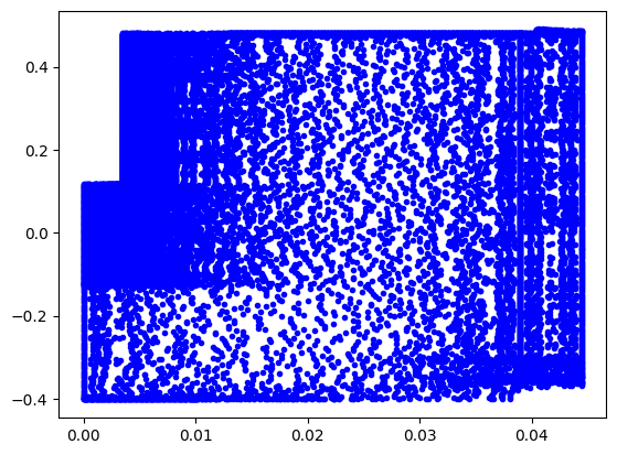
Temperature profile:
[4]:
X,Y = df['X (m)'], df['Y (m)']
fig = plt.figure(figsize=(5,8))
plt.scatter(X*100,Y*100, s=10, c=df['Temperature (K)'],cmap=plt.cm.coolwarm)
plt.xlabel('X (cm)')
plt.tick_params(axis='x', labelrotation = 90)
plt.ylabel('Y (cm)')
cbar = plt.colorbar()
cbar.set_label('Temperature ($^{\circ}K$)')
axes=plt.gca()
axes.set_aspect(0.7)

Data preprocessing, Wrangling, Cleansing and Scraping
[5]:
Responses = ['Temperature (K)','Velocity[i] (m/s)','Velocity[j] (m/s)']
RoI = Responses[0]
filename = "data/simulation_example_data/"
data = np.zeros((40510,49))
counter = -1
for j,i in enumerate(np.arange(350,700,50)):
    for l,k in enumerate(np.arange(240,450,30)):
        df = pd.read_csv(filename + str(i) + '_' + str(k) + '.csv')
        counter += 1
        if i == 650 and k == 420:
            print(counter)
        for n in range(3):
            df[Responses[n]].replace(to_replace='1.79769313486232e+308', value=0.0, inplace=True)
        data[:,counter] = df[RoI]
48
[6]:
data = data.T
print(np.shape(data))
df
(49, 40510)
[6]:
| Temperature (K) | Velocity[i] (m/s) | Velocity[j] (m/s) | X (m) | Y (m) | Z (m) | |
|---|---|---|---|---|---|---|
| 0 | 526.648511 | 0.0 | 0.0 | 0.002953 | -0.017654 | 0 |
| 1 | 526.645400 | 0.0 | 0.0 | 0.002982 | -0.017977 | 0 |
| 2 | 526.669124 | 0.0 | 0.0 | 0.002863 | -0.017775 | 0 |
| 3 | 526.738401 | 0.0 | 0.0 | 0.002503 | -0.017575 | 0 |
| 4 | 526.668918 | 0.0 | 0.0 | 0.002881 | -0.018116 | 0 |
| ... | ... | ... | ... | ... | ... | ... |
| 40505 | 420.000000 | 0.0 | 0.0 | 0.044450 | -0.237005 | 0 |
| 40506 | 420.000000 | 0.0 | 0.0 | 0.044450 | -0.239735 | 0 |
| 40507 | 420.000000 | 0.0 | 0.0 | 0.044450 | -0.242478 | 0 |
| 40508 | 420.000000 | 0.0 | 0.0 | 0.044450 | -0.245220 | 0 |
| 40509 | 420.000000 | 0.0 | 0.0 | 0.044450 | -0.247962 | 0 |
40510 rows × 6 columns
Find all sensor locations using built in QR optimizer
[7]:
n_sensors = 8
n_modes = 8
basis = ps.basis.SVD(n_basis_modes=n_modes)
optimizer  = ps.optimizers.QR()
model = ps.SSPOR(basis=basis, optimizer=optimizer, n_sensors=n_sensors)
model.fit(data)
all_sensors = model.get_all_sensors()
sensors = model.get_selected_sensors()
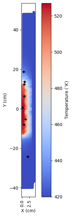
Sensor locations on the grid:
[8]:
yUnconstrained = df['Y (m)'][sensors]
xUnconstrained = df['X (m)'][sensors]

X,Y = df['X (m)'], df['Y (m)']
fig = plt.figure(figsize=(5,8))
plt.scatter(X*100,Y*100, s=10, c=df['Temperature (K)'],cmap=plt.cm.coolwarm)
plt.xlabel('X (cm)')
plt.tick_params(axis='x', labelrotation = 90)
plt.ylabel('Y (cm)')
cbar = plt.colorbar()
cbar.set_label('Temperature ($^{\circ}K$)')
plt.plot(xUnconstrained*100,yUnconstrained*100,'*k')
axes=plt.gca()
axes.set_aspect(0.7)
When working with dataframe data, you need to specify the column names for your axes: provide the x and y column names for 2D visualizations and constraint definitions, or x, y, and z column names for 3D visualizations and constraint definitions.
[9]:
xUnc, yUnc = ps.utils._constraints.get_coordinates_from_indices(sensors,df, Y_axis = 'Y (m)', X_axis = 'X (m)', Field = 'Temperature (K)')
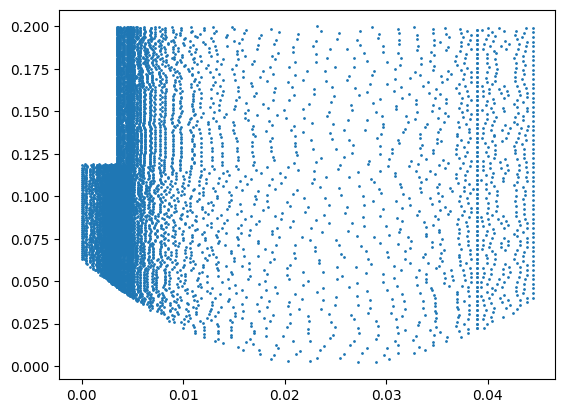
Functional constraints
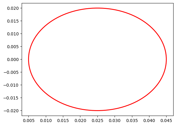
Suppose the user wants to constrain a circular area centered at \(x = 0.025\) m, \(y = 0\) m with a radius (\(r = 0.02\) m). The user can do see by initiating an instance of the class Circle which has functionalities such as :
Plotting
Plotting all possible sensor locations
Plotting the constraint on data
Obtaining indices of sensors within/outside the constrained circle
A dataframe of sensor indices along with their coordinate locations on the grid
Plotting the sensors on the grid
Annotating with the sensor number
[10]:
circle = ps.utils._constraints.Circle(center_x = 0.025, center_y = 0, radius = 0.02, loc = 'in', data = df, Y_axis = 'Y (m)', X_axis = 'X (m)', Field = 'Temperature (K)') #Plotting the constrained circle
circle.draw_constraint() ###Plotting just the constraint
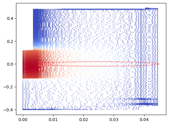
[11]:
circle.plot_constraint_on_data(plot_type='contour_map') ##Plotting the constraint on the data
[12]:
circle.plot_grid(all_sensors=all_sensors)
[13]:
const_idx, rank = circle.get_constraint_indices(all_sensors = all_sensors, info=df)
[14]:
# Define the number of constrained sensors allowed (s)
n_const_sensors = 1

# Define the GQR optimizer for the exact_n sensor placement strategy
optimizer_circle = ps.optimizers.GQR()
opt_exact_kws={'idx_constrained':const_idx,
         'n_sensors':n_sensors,
         'n_const_sensors':n_const_sensors,
         'all_sensors':all_sensors,
         'constraint_option':"exact_n"}
basis_exact = ps.basis.SVD(n_basis_modes=n_sensors)
[15]:
# Initialize and fit the model
model_exact = ps.SSPOR(basis = basis_exact, optimizer = optimizer_circle, n_sensors = n_sensors)
model_exact.fit(data,**opt_exact_kws)

# sensor locations based on columns of the data matrix
top_sensors_exact = model_exact.get_selected_sensors()

# sensor locations based on pixels of the image
xCircle, yCircle = ps.utils._constraints.get_coordinates_from_indices(top_sensors_exact,df,Y_axis = 'Y (m)', X_axis = 'X (m)', Field = 'Temperature (K)' )

print('The list of sensors selected is: {}'.format(top_sensors_exact))
The list of sensors selected is: [15658 18378 29993 16573 31414 40090 21456 37537]
[16]:
data_sens_circle = circle.sensors_dataframe(sensors = top_sensors_exact)
data_sens_circle
[16]:
| Sensor ID | SensorX | sensorY | |
|---|---|---|---|
| 0 | 15658.0 | 0.008200 | 0.136713 |
| 1 | 18378.0 | 0.006977 | 0.063449 |
| 2 | 29993.0 | 0.011413 | -0.051947 |
| 3 | 16573.0 | 0.007676 | 0.124104 |
| 4 | 31414.0 | 0.006206 | -0.079055 |
| 5 | 40090.0 | 0.019092 | -0.241529 |
| 6 | 21456.0 | 0.004899 | 0.187096 |
| 7 | 37537.0 | 0.005085 | -0.001238 |
[17]:
circle.plot_constraint_on_data(plot_type='contour_map')
# circle.plot_selected_sensors(sensors = top_sensors_exact, all_sensors=all_sensors)
circle.annotate_sensors(sensors = top_sensors_exact, all_sensors=all_sensors)
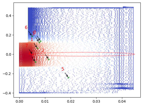
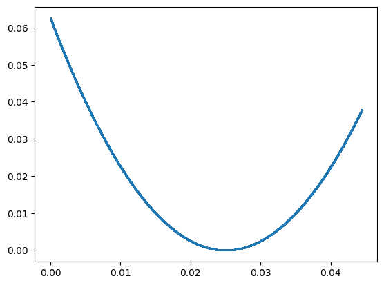
Custom parabolic constraint
Consider that a user has provided a python file with the required constraints.
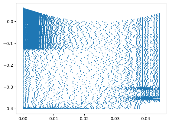
Here the parabola is centered at \((h,k) = (0.025,0.00)\). The equation used is \(y = a(x-h)^2 -k\) where \(a = 100\). A line drawn at \(y = 0.2\) closes the parabola and the constrained region is bound by the parabola and the line.
The user can initiate an instance of the class UserDefinedConstraints and use functionalities like plotting, annotating, creating a dataframe
[18]:
const5 = 'helper_scripts/twistParabolicConstraint.py' ### Python file with the required constraints
user_const_instance = ps.utils._constraints.UserDefinedConstraints(all_sensors, file = const5, data = df, Y_axis = 'Y (m)', X_axis = 'X (m)', Field = 'Temperature (K)' )
idx, rank = user_const_instance.constraint()
user_const_instance.draw_constraint() ## plot the user defined constraint just by itself
Using these constrained indices with pysensors GQR optimizer:
[19]:
# Define the number of constrained sensors allowed (s)
n_const_sensors = 0

# Define the GQR optimizer for the exact_n sensor placement strategy
optimizer_user = ps.optimizers.GQR()
opt_user_kws={'idx_constrained':idx,
         'n_sensors':n_sensors,
         'n_const_sensors':n_const_sensors,
         'all_sensors':all_sensors,
         'constraint_option':"exact_n"}
basis_user = ps.basis.SVD(n_basis_modes=n_sensors)
List of selected sensors
[20]:
# Initialize and fit the model
model_user = ps.SSPOR(basis = basis_user, optimizer = optimizer_user, n_sensors = n_sensors)
model_user.fit(data,**opt_user_kws)

# sensor locations based on columns of the data matrix
top_sensors_user = model_user.get_selected_sensors()

# sensor locations based on pixels of the image
# sensor locations based on pixels of the image
xCircle, yCircle = ps.utils._constraints.get_coordinates_from_indices(top_sensors_exact,df,Y_axis = 'Y (m)', X_axis = 'X (m)', Field = 'Temperature (K)' )

print('The list of sensors selected is: {}'.format(top_sensors_exact))
The list of sensors selected is: [15658 18378 29993 16573 31414 40090 21456 37537]
List of indices of sensors selected along with their coordinate locations on the grid
[21]:
data_sens_user = user_const_instance.sensors_dataframe(sensors = top_sensors_user)
data_sens_user
[21]:
| Sensor ID | SensorX | sensorY | |
|---|---|---|---|
| 0 | 31414.0 | 0.006206 | -0.079055 |
| 1 | 30106.0 | 0.011132 | -0.040648 |
| 2 | 19000.0 | 0.006517 | 0.033655 |
| 3 | 36479.0 | 0.010434 | -0.230693 |
| 4 | 35723.0 | 0.006281 | -0.377601 |
| 5 | 2620.0 | 0.000124 | -0.009141 |
| 6 | 21714.0 | 0.004854 | 0.200180 |
| 7 | 16921.0 | 0.000000 | 0.061600 |
The sensor locations plotted on the grid along with the constrained region
[22]:
user_const_instance.plot_constraint_on_data(plot_type='contour_map')
user_const_instance.plot_selected_sensors(sensors = top_sensors_user, all_sensors=all_sensors)
user_const_instance.annotate_sensors(sensors = top_sensors_user, all_sensors=all_sensors)
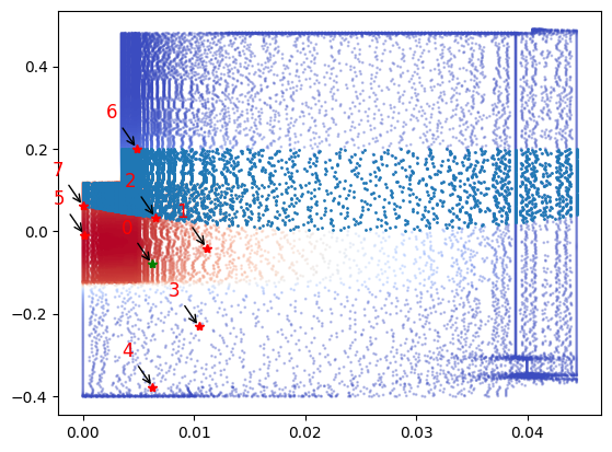
Now lets look at how to do the above with the constraint shapes defined in the class:
Initiating a class instance of the shape parabola :
[23]:
parabola = ps.utils._constraints.Parabola(h = 0.025, k = 0, a = 100, loc = 'in', data = df, Y_axis = 'Y (m)', X_axis = 'X (m)', Field = 'Temperature (K)') #Plotting the constrained circle
parabola.draw_constraint() ###Plotting just the constraint
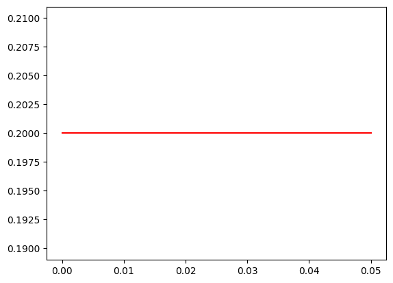
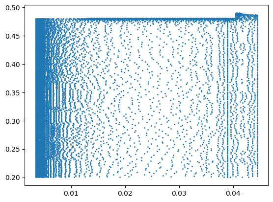
Initiating a class instance of the shape line :
[24]:
line1 = ps.utils._constraints.Line(x1 = 0, x2 = 0.05, y1 = 0.2, y2 = 0.2, data = df, Y_axis = 'Y (m)', X_axis = 'X (m)', Field = 'Temperature (K)') #Plotting the constrained line  ##expect a tuple of (x,y)
line1.draw_constraint() ## plotting just the constraint
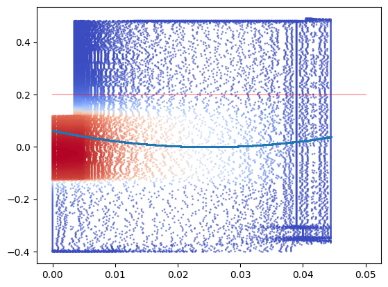
[25]:
fig , ax = plt.subplots()
line1.plot_constraint_on_data(plot_type='contour_map', plot= (fig,ax)) ## Plotting the constraint on the data
parabola.plot_constraint_on_data(plot_type='contour_map', plot = (fig,ax)) ## Plotting the constraint on the data
Locating constrained indices of the parabola
[26]:
const_idx_parabola, rank_parabola = parabola.get_constraint_indices(all_sensors=all_sensors, info = df)
Locating constrained indices of the line
[27]:
const_idx1, rank1 = line1.get_constraint_indices(all_sensors=all_sensors, info = df)
Finding the common constrained indices between them :
[28]:
Common_constrained_idx = np.intersect1d(const_idx_parabola, const_idx1)
Using the common constrained indices with the GQR optimizer in pysensors
[29]:
# Define the number of constrained sensors allowed (s)
n_const_sen_parabola = 0

# Define the GQR optimizer for the exact_n sensor placement strategy
optimizer_parabola = ps.optimizers.GQR()
opt_parabola_kws={'idx_constrained': Common_constrained_idx,
         'n_sensors':n_sensors,
         'n_const_sensors':n_const_sen_parabola,
         'all_sensors':all_sensors,
         'constraint_option':"exact_n"}
basis_parabola = ps.basis.SVD(n_basis_modes=n_sensors)
[30]:
# Initialize and fit the model
model_parabola = ps.SSPOR(basis = basis_parabola, optimizer = optimizer_parabola, n_sensors = n_sensors)
model_parabola.fit(data,**opt_parabola_kws)

# sensor locations based on columns of the data matrix
top_sensors_parabola = model_parabola.get_selected_sensors()

# sensor locations based on pixels of the image
xPara, yPara = ps.utils._constraints.get_coordinates_from_indices(top_sensors_parabola,df,Y_axis = 'Y (m)', X_axis = 'X (m)', Field = 'Temperature (K)' )

print('The list of sensors selected is: {}'.format(top_sensors_parabola))
The list of sensors selected is: [31414 30106 19000 36479 35723 2620 21714 16921]
[31]:
data_sens_parabola = parabola.sensors_dataframe(sensors = top_sensors_parabola)
data_sens_parabola
[31]:
| Sensor ID | SensorX | sensorY | |
|---|---|---|---|
| 0 | 31414.0 | 0.006206 | -0.079055 |
| 1 | 30106.0 | 0.011132 | -0.040648 |
| 2 | 19000.0 | 0.006517 | 0.033655 |
| 3 | 36479.0 | 0.010434 | -0.230693 |
| 4 | 35723.0 | 0.006281 | -0.377601 |
| 5 | 2620.0 | 0.000124 | -0.009141 |
| 6 | 21714.0 | 0.004854 | 0.200180 |
| 7 | 16921.0 | 0.000000 | 0.061600 |
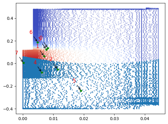
Sensor locations:
[32]:
parabola.plot_constraint_on_data(plot_type='contour_map') ## Plotting the constraint on the data!
parabola.plot_selected_sensors(sensors = top_sensors_parabola, all_sensors=all_sensors)
parabola.annotate_sensors(sensors = top_sensors_parabola, all_sensors=all_sensors)

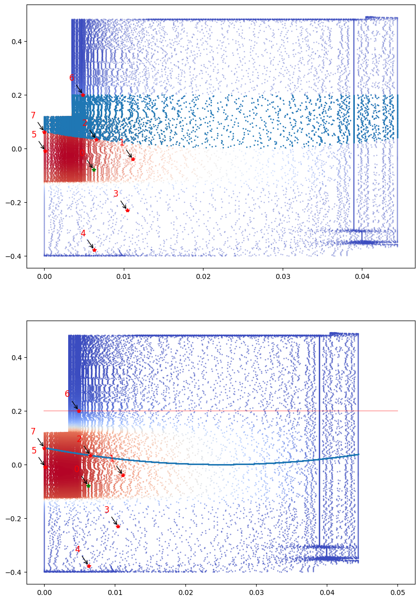
Lets compare the results we get from both methods:
[33]:
fig,ax = plt.subplots(2, figsize = (10,15))
user_const_instance.plot_constraint_on_data(plot_type='contour_map', plot = (fig,ax[0]))
user_const_instance.plot_selected_sensors(sensors = top_sensors_user, all_sensors=all_sensors)
user_const_instance.annotate_sensors(sensors = top_sensors_user, all_sensors=all_sensors)

line1.plot_constraint_on_data(plot_type= 'contour_map', plot = (fig,ax[1]))
parabola.plot_constraint_on_data(plot_type='contour_map', plot = (fig,ax[1])) ## Plotting the constraint on the data!
parabola.plot_selected_sensors(sensors = top_sensors_parabola, all_sensors=all_sensors)
parabola.annotate_sensors(sensors = top_sensors_parabola, all_sensors=all_sensors)
Now let us consider an example where the user inputs the equation that they are considering as a constraint in a string
For example the equation of a parabola is : \(a(x-h)^2 - (y- k)\)
[34]:
const5_stg = '(100*((x-0.025)**2)) > y' ### Python string with the required equation for a parabola
user_const_stg_instance = ps.utils._constraints.UserDefinedConstraints(all_sensors, data = df, Y_axis = 'Y (m)', X_axis = 'X (m)', Field = 'Temperature (K)' , equation = const5_stg)
idx_stg, rank_stg = user_const_stg_instance.constraint()
user_const_stg_instance.draw_constraint() ## plot the user defined constraint just by itself
And the equation of the line is : y - 0.2 = 0
[35]:
const5_line_stg = 'y > 0.2' ### Python string with the required equation for a parabola
user_const_stg_line_instance = ps.utils._constraints.UserDefinedConstraints(all_sensors, data = df, Y_axis = 'Y (m)', X_axis = 'X (m)', Field = 'Temperature (K)' , equation = const5_line_stg)
idx_stg_line, rank_stg_line = user_const_stg_line_instance.constraint()
user_const_stg_line_instance.draw_constraint() ## plot the user defined constraint just by itself
[36]:
#### Combining constrained indices for line and parabola:
Common_constrained_idx_stg = np.intersect1d(idx_stg_line, idx_stg)
[37]:
# Define the number of constrained sensors allowed (s)
n_const_sensors = 0

# Define the GQR optimizer for the exact_n sensor placement strategy
optimizer_user_stg = ps.optimizers.GQR()
opt_user_kws_stg={'idx_constrained':Common_constrained_idx_stg,
         'n_sensors':n_sensors,
         'n_const_sensors':n_const_sensors,
         'all_sensors':all_sensors,
         'constraint_option':"exact_n"}
basis_user_stg = ps.basis.SVD(n_basis_modes=n_sensors)
[38]:
# Initialize and fit the model
model_user_stg = ps.SSPOR(basis = basis_user_stg, optimizer = optimizer_user_stg, n_sensors = n_sensors)
model_user_stg.fit(data,**opt_user_kws_stg)

# sensor locations based on columns of the data matrix
top_sensors_user_stg = model_user_stg.get_selected_sensors()

# sensor locations based on pixels of the image
# sensor locations based on pixels of the image
xCircle_stg, yCircle_stg = ps.utils._constraints.get_coordinates_from_indices(top_sensors_exact,df,Y_axis = 'Y (m)', X_axis = 'X (m)', Field = 'Temperature (K)' )

print('The list of sensors selected is: {}'.format(top_sensors_user_stg))
The list of sensors selected is: [15658 18378 29993 16573 31414 40090 21456 7748]
[39]:
data_sens_user_stg = user_const_stg_instance.sensors_dataframe(sensors = top_sensors_user_stg)
data_sens_user_stg
[39]:
| Sensor ID | SensorX | sensorY | |
|---|---|---|---|
| 0 | 15658.0 | 0.008200 | 0.136713 |
| 1 | 18378.0 | 0.006977 | 0.063449 |
| 2 | 29993.0 | 0.011413 | -0.051947 |
| 3 | 16573.0 | 0.007676 | 0.124104 |
| 4 | 31414.0 | 0.006206 | -0.079055 |
| 5 | 40090.0 | 0.019092 | -0.241529 |
| 6 | 21456.0 | 0.004899 | 0.187096 |
| 7 | 7748.0 | 0.000192 | 0.005811 |
[40]:
user_const_stg_instance.plot_constraint_on_data(plot_type='contour_map')
user_const_stg_instance.plot_selected_sensors(sensors = top_sensors_user_stg, all_sensors=all_sensors)
user_const_stg_instance.annotate_sensors(sensors = top_sensors_user_stg, all_sensors = all_sensors)
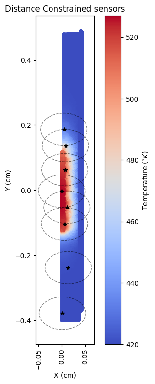
Distance constrained
Let us consider an example where sensors need to be placed at a \(r=0.05\) metres from each other.
[41]:
r = 0.05
optimizer_distance= ps.optimizers.GQR()
opt_distance_kws ={
         'n_sensors':n_sensors,
         'all_sensors':all_sensors,
         'r': r,
         'info': df,
         'X_axis': 'X (m)',
         'Y_axis': 'Y (m)',
         'constraint_option':"distance"}
basis_distance = ps.basis.SVD(n_basis_modes=n_sensors)
[42]:
# Initialize and fit the model
model_distance = ps.SSPOR(basis = basis_distance, optimizer = optimizer_distance, n_sensors = n_sensors)
model_distance.fit(data,**opt_distance_kws)

# sensor locations based on columns of the data matrix
top_sensors_distance = model_distance.get_selected_sensors()

xdistance, ydistance = ps.utils._constraints.get_coordinates_from_indices(top_sensors_exact,df,Y_axis = 'Y (m)', X_axis = 'X (m)', Field = 'Temperature (K)' )

print('The list of sensors selected is: {}'.format(top_sensors_distance))
The list of sensors selected is: [15658 18378 29993 30516 40091 1769 21456 35709]
[43]:
from matplotlib.patches import Circle
fig = plt.figure(figsize=(5, 8))
plt.scatter(X, Y, s=10, c=df['Temperature (K)'], cmap=plt.cm.coolwarm)
plt.xlabel('X (cm)')
plt.tick_params(axis='x', labelrotation=90)
plt.ylabel('Y (cm)')
cbar = plt.colorbar()
cbar.set_label('Temperature ($^{\circ}K$)')
plt.title('Distance Constrained sensors')

xdistance_values = []
ydistance_values = []
for idx in top_sensors_distance:
    xdistance_values.append(df.loc[idx, 'X (m)'])
    ydistance_values.append(df.loc[idx, 'Y (m)'])

xdistance_array = np.array(xdistance_values)
ydistance_array = np.array(ydistance_values)

plt.plot(xdistance_array, ydistance_array, '*k')

ax = plt.gca()

for i in range(len(xdistance_array)):
    circ = Circle((xdistance_array[i], ydistance_array[i]), r,
                  color='k', fill=False, alpha=0.5, linestyle='--')
    ax.add_patch(circ)

# Set aspect ratio
ax.set_aspect(0.7)
plt.tight_layout()
plt.show()