Cross-validation

This notebook shows how to use cross-validation techniques from Scikit-learn to tune parameters.

Note that the pandas package is required to run this notebook.

import matplotlib.pyplot as plt
import numpy as np
import pandas as pd
import seaborn as sns
from sklearn import datasets

import pysensors as ps

Setup

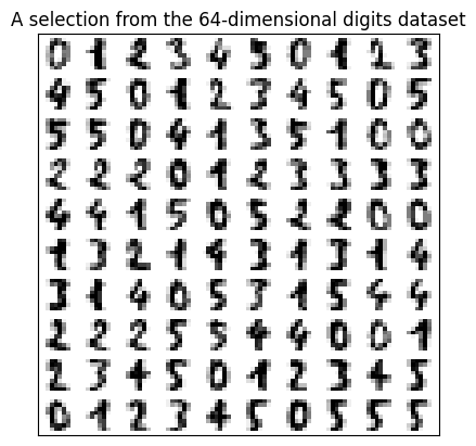
First we’ll load some training data. In this case, images of handwritten digits.

digits = datasets.load_digits(n_class=6)
X = digits.data
y = digits.target

n_samples, n_features = X.shape
print(n_samples, n_features)

1083 64

# Plot some digits
n_img_per_row = 10
img = np.zeros((10 * n_img_per_row, 10 * n_img_per_row))
for i in range(n_img_per_row):
    ix = 10 * i + 1
    for j in range(n_img_per_row):
        iy = 10 * j + 1
        img[ix:ix + 8, iy:iy + 8] = X[i * n_img_per_row + j].reshape((8, 8))

plt.imshow(img, cmap=plt.cm.binary)
plt.xticks([])
plt.yticks([])
plt.title('A selection from the 64-dimensional digits dataset')
plt.show()

Grid search

Here we specify a set of parameter values we’d like to test. The GridSearchCV object will try out every possible combination and tell us which gave the best performance.

from sklearn.model_selection import GridSearchCV

model = ps.reconstruction.SSPOR()

param_grid = {
    "basis": [ps.basis.Identity(), ps.basis.SVD(), ps.basis.RandomProjection()],
    "basis__n_basis_modes": [20, 30, 40, 50],
    "n_sensors": [10, 20, 30, 40]
}

search = GridSearchCV(model, param_grid)
search.fit(X, quiet=True)
print("Best parameters:")
for k, v in search.best_params_.items():
    print(f"{k}:  {v}")

Best parameters:
basis:  SVD(n_basis_modes=40)
basis__n_basis_modes:  40
n_sensors:  40

We can also visualize the performance of each candidate model to get a better idea how the different parameters interact. The pandas and seaborn packages help simplify the task.

def rename_bases(s):
        if 'Identity' in str(s):
            return 'Identity'
        elif 'SVD' in str(s):
            return 'SVD'
        elif 'RandomProjection' in str(s):
            return 'RandomProjection'
        else:
            return "N/A"

def create_dataframe(results):
    results_df = pd.DataFrame.from_dict(results)

    # Rename the basis objects for plotting purposes
    results_df['basis'] = results_df['param_basis'].apply(rename_bases)

    # We were working with the negative mean-square error before
    results_df['neg_mean_test_score'] = -results_df['mean_test_score']

    return results_df

def generate_summary_plots(results):
    results = create_dataframe(results)

    fig, axs = plt.subplots(1, 2, figsize=(14, 6))
    sns.barplot(data=results, x='param_basis__n_basis_modes', y='neg_mean_test_score', hue='basis', ax=axs[0])
    sns.barplot(data=results, x='param_n_sensors', y='neg_mean_test_score', hue='basis', ax=axs[1])
    axs[0].set(xlabel='n_basis_modes', ylabel='Mean square error')
    axs[1].set(xlabel='n_sensors', ylabel='Mean square error');

generate_summary_plots(search.cv_results_)

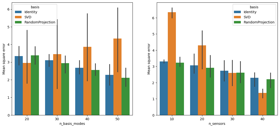
The error bars in the left subplot come from different choices of n_sensors. Those on the right come from different values of n_basis_modes. Note that the performance of the SVD basis is more sensitive to low sensor counts than the other two bases, but it does very well once enough sensors are in place.

We can also look more closely at how the different bases are affected by differing numbers of sensors.

# Rename basis objects
results = create_dataframe(search.cv_results_)

# Initialize a grid with a plot for each number of basis modes
grid = sns.FacetGrid(results, col="param_basis__n_basis_modes", hue="basis", legend_out=False)

# Create a plot for each instance
grid.map(plt.plot, "param_n_sensors", "neg_mean_test_score", marker="o").add_legend()
grid.fig.tight_layout()
plt.show()

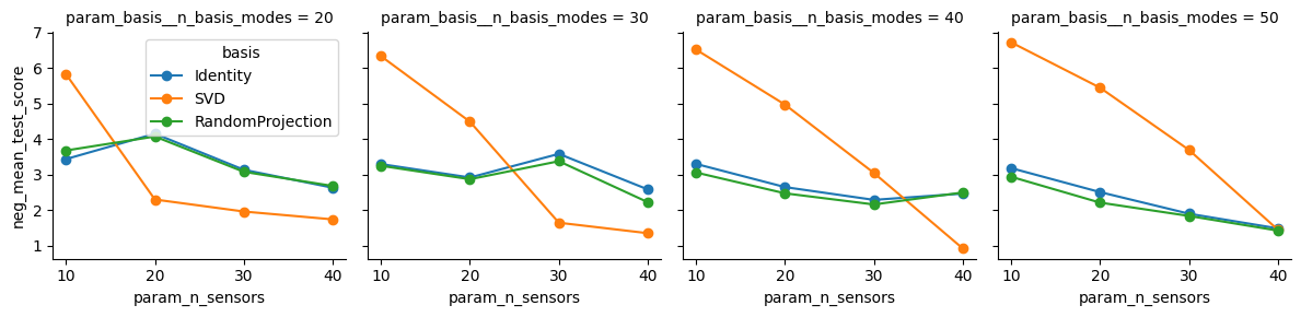
• SVD - Performance generally increases as the number of sensors are increased. For low sensor counts, this basis is beat out by the other two.

• Identity - Works best when lots of modes are retained, even for low values of n_sensors.

• RandomProjection - Similar performance to the Identity basis on this example.

Randomized search

Now suppose we have a fixed sensor budget. We’d like to determine the best basis in which to represent the data to make the most of these sensors. Suppose further that we want to test out a larger number of candidates for n_basis_modes. We can obtain a good approximation to the optimal parameter configuration for a fraction of the cost using Scikit-learn’s RandomizedSearchCV object.

from scipy.stats import randint
from sklearn.model_selection import RandomizedSearchCV

model = ps.reconstruction.SSPOR(n_sensors=30)

param_distributions = {
    "basis": [ps.basis.Identity(), ps.basis.SVD(), ps.basis.RandomProjection()],
    "basis__n_basis_modes": randint(10, 50)
}

search = RandomizedSearchCV(model, param_distributions, n_iter=30)
search.fit(X, quiet=True)
for k, v in search.best_params_.items():
    print(f"{k}:  {v}")

basis:  SVD(n_basis_modes=22)
basis__n_basis_modes:  22

results = pd.DataFrame.from_dict(search.cv_results_)

# Rename the basis objects for plotting purposes
def rename_bases(s):
    if 'Identity' in str(s):
        return 'Identity'
    elif 'SVD' in str(s):
        return 'SVD'
    elif 'RandomProjection' in str(s):
        return 'RandomProjection'
    else:
        return "N/A"

results['basis'] = results['param_basis'].apply(rename_bases)

# We were working with the negative mean-square error before
results['neg_mean_test_score'] = -results['mean_test_score']

fig, ax = plt.subplots(1, 1, figsize=(8, 6))
sns.lineplot(
    markers=True,
    data=results,
    x='param_basis__n_basis_modes',
    y='neg_mean_test_score',
    hue='basis',
    ax=ax
)
ax.set(xlabel='n_basis_modes', ylabel='Mean square error', title='30 sensors');

The Identity and RandomProjection bases appear to benefit from increasing the number of basis modes. Once the number of basis modes exceeds the number of sensors, the performance of the SVD basis drops off. Its accuracy curve shows that it is adept at compressing information as it attains good scores for low numbers of basis modes.

Note that the basis is recomputed for each value of n_basis_modes, which may create misleading results for the RandomProjection basis. Normally to increase the size of the basis one would simply add a new randomly projection vector to the existing basis, in which case we would expect to see something much closer to a monotonoic decrease in mean-square error in as n_basis_modes is increased.

See this notebook for a more in-depth comparison of the bases.

Download python script: cross_validation.py

Download Jupyter notebook: cross_validation.ipynb