PySensors Overview
This notebook is meant to give an overview of the basic functionality of PySensors. See our other notebooks for more detailed information about different methods and tasks.
Given measurement data PySensors helps one choose a sparse set of sensor locations for either reconstruction (interpolation) or classification. PySensors was written to be fully compatible with Scikit-learn. As such, most of its objects are Scikit-learn estimators, expecting training data to be numpy arrays with rows corresponding to examples and columns to features. Throughout PySensors it is typically assumed that different features (columns of measurement data)
correspond to different sensors or sensor locations.
For examples showing how to perform cross-validation with Scikit-learn and PySensors objects, see this notebook.
[1]:
import matplotlib.pyplot as plt
import numpy as np
from sklearn import datasets
from sklearn import metrics
from sklearn.model_selection import train_test_split

import pysensors as ps
[2]:
# Seed for reproducibility
random_state = 99
Reconstruction
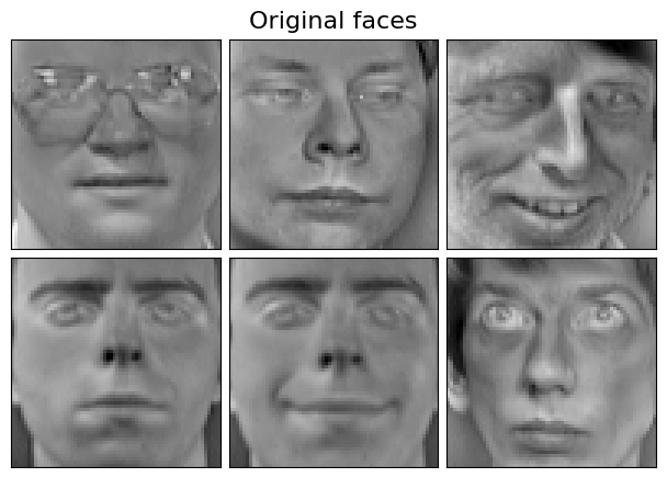
For our reconstruction examples we will consider the Olivetti faces dataset from AT&T, consisting of 10 64-by-64 pictures of 40 different people. Each pixel will be treated as a sensor. An additional example performing sensor selection with PySensors to approximate global sea surface temperatures is given here
For reconstruction PySensors provides the SSPOR class (Sparse Sensor Placement Optimization for Reconstruction), which is largely based on the following paper (link):
Manohar, Krithika, et al. "Data-driven sparse sensor placement for reconstruction: Demonstrating the benefits of exploiting known patterns." IEEE Control Systems Magazine 38.3 (2018): 63-86.
SSPOR objects can be imported directly from pysensors or from pysensors.reconstruction.
Setup
[3]:
faces = datasets.fetch_olivetti_faces(shuffle=True, random_state=random_state)
X = faces.data

n_samples, n_features = X.shape
print('Number of samples:', n_samples)
print('Number of features (sensors):', n_features)

# Global centering
X = X - X.mean(axis=0)

# Local centering
X -= X.mean(axis=1).reshape(n_samples, -1)

X_train, X_test = X[:300], X[300:]
Number of samples: 400
Number of features (sensors): 4096
[4]:
# From https://scikit-learn.org/stable/auto_examples/decomposition/plot_faces_decomposition.html
n_row, n_col = 2, 3
n_components = n_row * n_col
image_shape = (64, 64)

def plot_gallery(title, images, n_col=n_col, n_row=n_row, cmap=plt.cm.gray):
    '''Function for plotting faces'''
    plt.figure(figsize=(2. * n_col, 2.26 * n_row))
    plt.suptitle(title, size=16)
    for i, comp in enumerate(images):
        plt.subplot(n_row, n_col, i + 1)
        vmax = max(comp.max(), -comp.min())
        plt.imshow(comp.reshape(image_shape), cmap=cmap,
                   interpolation='nearest',
                   vmin=-vmax, vmax=vmax)
        plt.xticks(())
        plt.yticks(())
    plt.subplots_adjust(0.01, 0.05, 0.99, 0.93, 0.04, 0.)
[5]:
plot_gallery("First few centered faces", X[:n_components])

Simplest case
A SSPOR object is instantiated and fit to the data to obtain a ranking of sensors (technically sensor indices) in descending order of importance. We print the top 10 here.
[6]:
model = ps.SSPOR()
model.fit(X_train)

# Ranked list of sensors
ranked_sensors = model.get_selected_sensors()
print(ranked_sensors[:10])
[4032 4092 320 4039 2209 575 529 2331 878 2837]
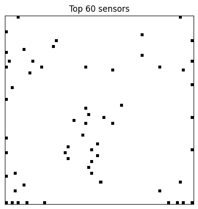
Here we visualize the locations of the top 60 sensors.
[7]:
# Plot the top 60 sensors
n_sensors = 60
fig, ax = plt.subplots(1, 1, figsize=(5, 5))

img = np.zeros(n_features)
img[ranked_sensors[:n_sensors]] = 16

ax.imshow(img.reshape(image_shape), cmap=plt.cm.binary)
ax.set(title=f'Top {n_sensors} sensors', xticks=[], yticks=[]);
Changing the number of sensors
Since we didn’t specify the number of sensors, SSPOR.get_selected_sensors() returned them all. Instead we can pass in the desired number of sensors when instantiating a SSPOR object or after it has been fitted. Both options yield the same result.
[8]:
# Set number of sensors after fitting
model.set_number_of_sensors(n_sensors)

# Set number of sensors before fitting
model_alt = ps.SSPOR(n_sensors=n_sensors)
model_alt.fit(X_train)

print('Number of sensors originally returned:', len(ranked_sensors))
print('Number of returned sensors after updating:', len(model.get_selected_sensors()))

assert all(model.get_selected_sensors() == model_alt.get_selected_sensors())
Number of sensors originally returned: 4096
Number of returned sensors after updating: 60
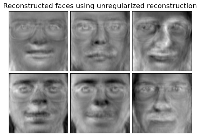
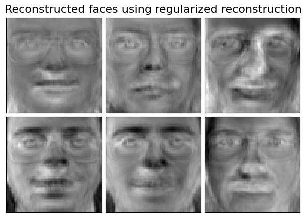
Forming reconstructions
Once a SSPOR model has been fit to the data, it can be used to form reconstructions based on measurements from the selected sensor locations. There are two ways of reconstruction, unregularized reconstruction and regularized reconstruction.
[9]:
# Fit the model
n_sensors = 60
model = ps.SSPOR(n_sensors=n_sensors).fit(X_train)

# Get the chosen sensor locations
sensors = model.get_selected_sensors()

# Subsample data so we only have measurements at chosen sensor locations
X_test_subsampled = X_test[:, sensors]

# Form reconstructions
X_test_unregularized_reconstructed = model.predict(X_test_subsampled, method='unregularized')
flat = np.full(300, 4)
X_test_regularized_reconstructed = model.predict(X_test_subsampled, method=None, prior=flat, noise=0.01)

plot_gallery("Original faces", X_test[:n_components])
plot_gallery("Reconstructed faces using unregularized reconstruction", X_test_unregularized_reconstructed[:n_components])
plot_gallery("Reconstructed faces using regularized reconstruction", X_test_regularized_reconstructed[:n_components])
Sweeping over a range of sensor counts
It is often useful to measure the reconstruction error as a function of the number of sensors.
Note that the error tends to spike when the number of sensors is close to the total number of examples (or the number of basis modes); in this case 300.
Another example of this functionality is given here.
[10]:
model = ps.SSPOR().fit(X_train)

sensor_range = np.arange(1, 1000, 10)
errors = model.reconstruction_error(X_test, sensor_range=sensor_range)

plt.plot(sensor_range, errors, '-o')
plt.xlabel('Number of sensors')
plt.ylabel('Reconstruction error (MSE)')
plt.title('Reconstruction error for different numbers of sensors');

Changing the basis
PySensors currently provides three choices of basis in which to represent measurement data:
Identity: uses the raw measurements (the default option)SVD: Singular Value Decomposition modes (equivalent to PCA modes if the data are centered)RandomProjection: Random Gaussian projections of the data
These classes are all contained in the pysensors.basis submodule. For a comparison of these options see this notebook.
[11]:
n_basis_modes = 20
SVD basis
[12]:
basis = ps.basis.SVD(n_basis_modes=n_basis_modes)
model = ps.SSPOR(basis=basis)
model.fit(X_train)

# Ranked list of sensors
svd_ranked_sensors = model.get_selected_sensors()
print('Original ranked sensors:', ranked_sensors[:10])
print('SVD ranked sensors:', svd_ranked_sensors[:10])
Original ranked sensors: [4032 4092  320 4039 2209  575  529 2331  878 2837]
SVD ranked sensors: [2209  319 3970  384 3034  594 4092 2331 2813 2839]
Random projections
[13]:
basis = ps.basis.RandomProjection(n_basis_modes=n_basis_modes)
model = ps.SSPOR(basis=basis)
model.fit(X_train)

# Ranked list of sensors
rp_ranked_sensors = model.get_selected_sensors()
print('Original ranked sensors:', ranked_sensors[:10])
print('Random projection ranked sensors:', rp_ranked_sensors[:10])
Original ranked sensors: [4032 4092  320 4039 2209  575  529 2331  878 2837]
Random projection ranked sensors: [ 256 3259 4034  555 2771 3096 3977  642 4087 2847]
Custom Basis
In this case, we create a random matrix and pass it on as a custom basis.
[14]:
U = np.random.randint(10, 20, (4096, 30))
basis = ps.basis.Custom(U=U)
model = ps.SSPOR(basis=basis)
model.fit(X_train)

# Ranked list of sensors
custom_ranked_sensors = model.get_selected_sensors()
print('Original ranked sensors:', ranked_sensors[:10])
print('Custom ranked sensors:', rp_ranked_sensors[:10])
Original ranked sensors: [4032 4092  320 4039 2209  575  529 2331  878 2837]
Custom ranked sensors: [ 256 3259 4034  555 2771 3096 3977  642 4087 2847]
Updating the number of basis modes
The number of basis modes can be updated after a SSPOR model has been fit via the update_n_basis_modes function.
Note that when using update_n_basis_modes to increase the number of basis modes from the number specified when the model was fit requires one to pass in the training data. The number of basis modes can be decreased without the need for the training data.
[15]:
# Decreasing the number of basis modes
basis = ps.basis.SVD(n_basis_modes=20)
model = ps.SSPOR(basis=basis).fit(X_train)
model.update_n_basis_modes(10, x=X_train)

# Increasing the number of basis modes
basis = ps.basis.SVD(n_basis_modes=20)
model = ps.SSPOR(basis=basis).fit(X_train)
model.update_n_basis_modes(30, x=X_train)
Changing the Optimizer
Pysensors has four choices of optimizers
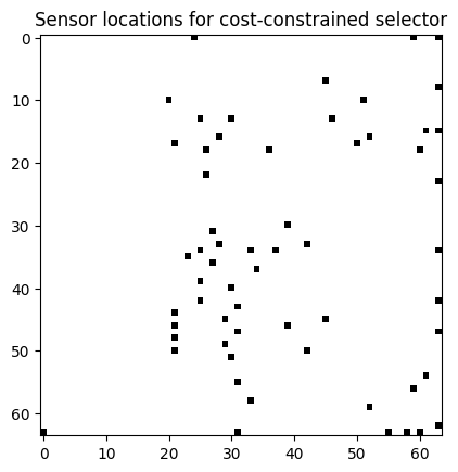
Cost-constraints
For many applications sensors impose non-uniform costs depending on their locations. For example, if we wanted to place sensors around the planet to estimate temperatures at every point on Earth, it would be more expensive (financially) to set up sensors in Antarctica than in Seattle. However, some sensor locations may provide enough information to outweigh this cost.
To handle cost-constrained sensor selection problems, PySensors provides the CCQR (cost-constrained QR) optimization method. One simply instantiates a CCQR object and passes it a vector of sensor costs. More examples are available in this notebook.
See the following reference for the mathematical details (link):
Clark, Emily, et al. "Greedy sensor placement with cost constraints." IEEE Sensors Journal 19.7 (2018): 2642-2656.
[16]:
# Define cost array
costs = np.zeros(image_shape)
costs[:, :20] = 1

plt.imshow(costs, vmin=0, vmax=1, cmap=plt.cm.gray)
plt.title('Cost array');

[17]:
costs = costs.reshape(-1)

# Fit the cost-constrained model
optimizer = ps.optimizers.CCQR(sensor_costs=costs)
model = ps.SSPOR(optimizer=optimizer, n_sensors=n_sensors)
model.fit(X_train)

# Visualize the top sensors
top_sensors = model.get_selected_sensors()
img = np.zeros(n_features)
img[top_sensors] = 16
plt.imshow(img.reshape(image_shape), cmap=plt.cm.binary)
plt.title('Sensor locations for cost-constrained selector');
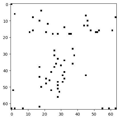
Spatial Consraints
Some applications allow for only a limited number of sensors, where predetermined locations are present, or restricted areas exist to disallow sensor placement. The General QR algorithm is used to address these problems. A detailed example is provided in this notebook.
Different types of spatial constraints
See the following reference for more information (link)
Niharika Karnik, Mohammad G. Abdo, Carlos E. Estrada Perez, Jun Soo Yoo, Joshua J. Cogliati, Richard S. Skifton, Pattrick Calderoni, Steven L. Brunton, and Krithika Manohar. Optimal Sensor Placement with Adaptive Constraints for Nuclear Digital Twins. 2023. arXiv: 2306 . 13637 [math.OC].
[18]:
xmin = 10
xmax = 30
ymin = 20
ymax = 40
all_sensors = model.get_all_sensors()
sensors_constrained = ps.utils._constraints.get_constrained_sensors_indices(
    xmin, xmax, ymin, ymax, image_shape[0], image_shape[1], all_sensors
)

n_const_sensors = 2
optimizer_exact = ps.optimizers.GQR()
opt_exact_kws = {
    "idx_constrained": sensors_constrained,
    "n_sensors": n_sensors,
    "n_const_sensors": n_const_sensors,
    "all_sensors": all_sensors,
    "constraint_option": "exact_n",
}
basis_exact = ps.basis.SVD(n_basis_modes=n_sensors)
model_exact = ps.SSPOR(
    basis=basis_exact, optimizer=optimizer_exact, n_sensors=n_sensors
)
model_exact.fit(X_train, **opt_exact_kws)
top_sensors = model_exact.get_selected_sensors()
Here, the region \(10 \leq x \leq 30\) and \(20 \leq y\leq 40\) is constrained such that it can only contain two sensors.
[19]:
img = np.zeros(n_features)
img[top_sensors] = 16
plt.plot([xmin, xmin], [ymin, ymax], "-.r")
plt.plot([xmin, xmax], [ymax, ymax], "-.r")
plt.plot([xmax, xmax], [ymin, ymax], "-.r")
plt.plot([xmin, xmax], [ymin, ymin], "-.r")
plt.imshow(img.reshape(image_shape), cmap=plt.cm.binary)
[19]:
<matplotlib.image.AxesImage at 0x7f3566f5c080>

Two Point Greedy Algorithm
For \(p\) sensors and \(r\) basis modes, while the QR optimizer returned exactly \(p=r\) sensors in order of decreasing importance through pivoting and placed any subsequent sensors randomly, a TPGR optimizer can return a user specified \(p\) sensors for any number of basis modes \(r\). This notebook goes into deeper detail about this optimizer.
See the following reference for more information on Regularized Least Squares Reconstruction and Two-Point Greedy Optimizer (link)
Klishin, Andrei A., J. Nathan Kutz and Krithika Manohar. Data-Induced Interactions of Sparse Sensors. 2023. arXiv:2307.11838 [cond-mat.stat-mech]
[20]:
optimizer = ps.optimizers.TPGR(n_sensors=n_sensors, noise=0.01)
model = ps.SSPOR(optimizer=optimizer)
model.fit(X_train)

top_sensors = model.get_selected_sensors()
img = np.zeros(n_features)
img[top_sensors] = 16
plt.imshow(img.reshape(image_shape), cmap=plt.cm.binary)
[20]:
<matplotlib.image.AxesImage at 0x7f3566fc3fe0>
Classification
For the classification examples we will consider the digits dataset. Each example consists of an 8-by-8 image of a handwritten digit. The goal is to train a model to identify which digit is written in a given image. In-depth examples are given in the classification notebook.
PySensors implements the Sparse Sensor Placement Optimization for Classification (SSPOC) algorithm in the SSPOC class. See the original SSPOC paper for more information (link):
Brunton, Bingni W., et al. "Sparse sensor placement optimization for classification." SIAM Journal on Applied Mathematics 76.5 (2016): 2099-2122.
SSPOC can be imported directly from pysensors or from pysensors.classification.
[21]:
from pysensors import SSPOC
[22]:
# Load data
digits = datasets.load_digits(n_class=10)
X = digits.data
y = digits.target

n_samples, n_features = X.shape

X_train, X_test, y_train, y_test = train_test_split(
    X, y, test_size=0.25, random_state=random_state
)

# Plot some digits
n_img_per_row = 10
img = np.zeros((10 * n_img_per_row, 10 * n_img_per_row))
for i in range(n_img_per_row):
    ix = 10 * i + 1
    for j in range(n_img_per_row):
        iy = 10 * j + 1
        img[ix:ix + 8, iy:iy + 8] = X[i * n_img_per_row + j].reshape((8, 8))

plt.imshow(img, cmap=plt.cm.binary)
plt.xticks([])
plt.yticks([])
plt.title('A selection from the 64-dimensional digits dataset')
plt.show()

print('Number of samples:', n_samples)
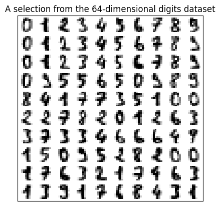
Number of samples: 1797
Simplest case
[23]:
model = SSPOC()
model.fit(X_train, y_train)

print('Portion of sensors used:', len(model.selected_sensors) / n_features)
print('Selected sensors:', model.selected_sensors)
Portion of sensors used: 0.0625
Selected sensors: [16 24 31 48]
Changing the number of sensors
There are a few methods of changing the number of sensors for SSPOC objects:
Specify
n_sensorswhen instantiating the model.Change the
l1_penaltyparameter. This affects the strength of the regularization applied when finding sensor locations. Ifn_sensorsis not passed to theSSPOCconstructor, then the value ofl1_penaltycan affect the number of sensors that are selected. You can also tune thethresholdparameter to further affect the sensor count.Update
n_sensorsafter fitting. Use theupdate_sensorsfunction to do so. It is recommended that you also pass in the training and test data so that the classifier can be refit using the new sensors.
See the classification notebook for more information.
[24]:
# Method 1
model = SSPOC(n_sensors=10).fit(X_train, y_train, quiet=True)
print('Portion of sensors used:', len(model.selected_sensors) / n_features)
print('Selected sensors:', model.selected_sensors)
Portion of sensors used: 0.15625
Selected sensors: [24 48 16 31  4  1  2  0  8  9]
[25]:
# Method 2 - only works for multiclass classification problems
model = SSPOC(l1_penalty=0.01).fit(X_train, y_train)
print('Portion of sensors used (default threshold):', len(model.selected_sensors) / n_features)
print('Selected sensors:', model.selected_sensors)

# Tune threshold to affect number of sensors chosen
model = SSPOC(threshold=1, l1_penalty=0.01).fit(X_train, y_train)
print('\n')
print('Portion of sensors used (higher threshold):', len(model.selected_sensors) / n_features)
print('Selected sensors:', model.selected_sensors)
Portion of sensors used (default threshold): 0.59375
Selected sensors: [ 1  3  5  6  7  8 10 12 15 16 18 20 21 22 23 24 30 31 33 38 40 41 42 43
 44 45 46 47 48 49 52 53 55 57 60 61 62 63]


Portion of sensors used (higher threshold): 0.140625
Selected sensors: [ 8 15 16 23 24 31 40 47 48]
[26]:
# Method 3 - update after fitting
model = SSPOC().fit(X_train, y_train)
model.update_sensors(n_sensors=10, xy=(X_train, y_train), quiet=True)
print('Portion of sensors used:', len(model.selected_sensors) / n_features)
print('Selected sensors:', model.selected_sensors)
Portion of sensors used: 0.15625
Selected sensors: [24 48 16 31  4  1  2  0  8  9]
Changing the basis
Like the SSPOR object, SSPOC instances accept a basis argument.
[27]:
basis = ps.basis.SVD(n_basis_modes=10)
model = SSPOC(basis=basis).fit(X_train, y_train)
print('Portion of sensors used:', len(model.selected_sensors) / n_features)
print('Selected sensors:', model.selected_sensors)
Portion of sensors used: 1.0
Selected sensors: [ 0  1  2  3  4  5  6  7  8  9 10 11 12 13 14 15 16 17 18 19 20 21 22 23
 24 25 26 27 28 29 30 31 32 33 34 35 36 37 38 39 40 41 42 43 44 45 46 47
 48 49 50 51 52 53 54 55 56 57 58 59 60 61 62 63]
Changing the classifier
Additionally, one has the option to specify the classifier the SSPOC object uses. Any linear classifier with fit and predict methods and a coef_ attribute are compatible.
[28]:
from sklearn.linear_model import SGDClassifier

classifier = SGDClassifier(max_iter=5000, loss='modified_huber', random_state=random_state)
model = SSPOC(classifier=classifier, n_sensors=10).fit(X_train, y_train, quiet=True)
print('Portion of sensors used:', len(model.selected_sensors) / n_features)
print('Selected sensors:', model.selected_sensors)
Portion of sensors used: 0.15625
Selected sensors: [43 53 12 28 61 27 26 30 52 42]
Measuring accuracy
Once fit, SSPOC objects can also be used to make class predictions.
The predict method transforms the (subsampled) data to the appropriate basis, then applies the classifier to obtain predicted labels. These can then be used to check the accuracy of the model on the test set.
[29]:
y_pred = model.predict(X_test[:, model.selected_sensors])
print('Test set accuracy:', metrics.accuracy_score(y_test, y_pred))
Test set accuracy: 0.78